Key Takeaways
- Hiding rows & columns in Google Sheets declutters your spreadsheet for easier digestion.
- Hiding affects entire row or column —move data to keep visible before hiding.
- Unhide rows & columns by clicking arrows or right-clicking adjacent cells, maintaining functionality.
Less is more. This saying doesn’t always apply to the amount of data in your Google Sheets—there, more can indeed be more. But when it comes to presenting this data, less is definitely better. Hiding columns and rows that are necessary for calculations but not for presentation can work wonders in decluttering your spreadsheet and make it easier to digest.
How to Hide Rows and Columns in Google Sheets
When you hide a row or column, it remains in your spreadsheet, fully functional and still part of any calculations. The only difference is that you won’t see it.
Remember that hiding affects the entire row or column. If there’s data you still want to keep visible, move it elsewhere before hiding.
Hiding rows or columns in Google Sheets is straightforward. Select the row or column, right-click, and choose Hide from the menu.
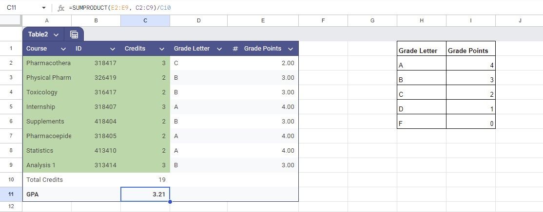
For example, in a spreadsheet where I calculated my GPA for a heavy semester, I created a guide table with grade point equivalents (e.g., A = 4 points). This table is crucial for my calculations, but otherwise, I don’t need to see it. So, let’s hide it.
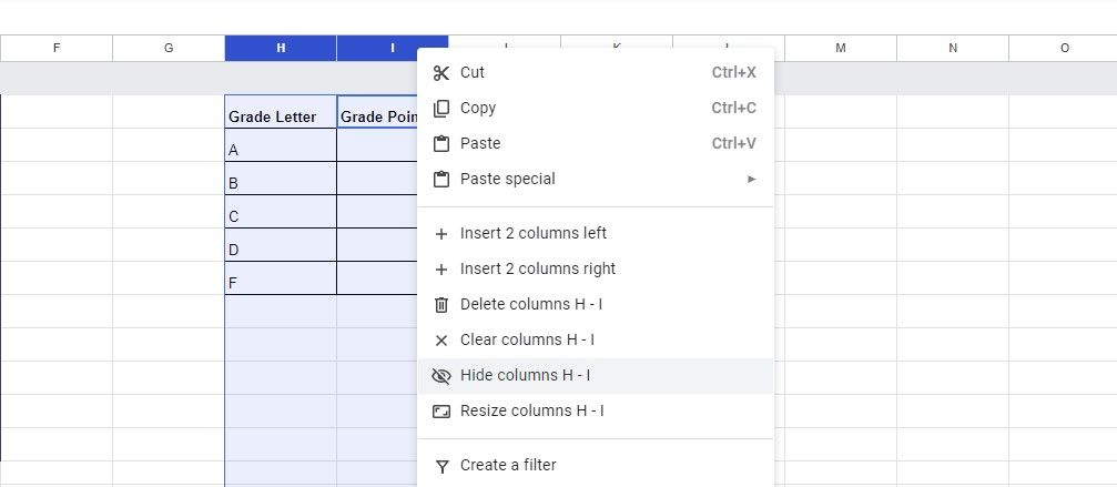
The table spans columns H and I. To hide columns in Google Sheets, select both columns by holding Ctrl and clicking each one, then right-click and choose Hide columns.
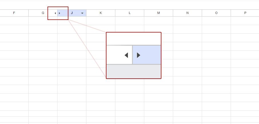
The columns disappear, leaving only two tiny arrows indicating their hidden location.
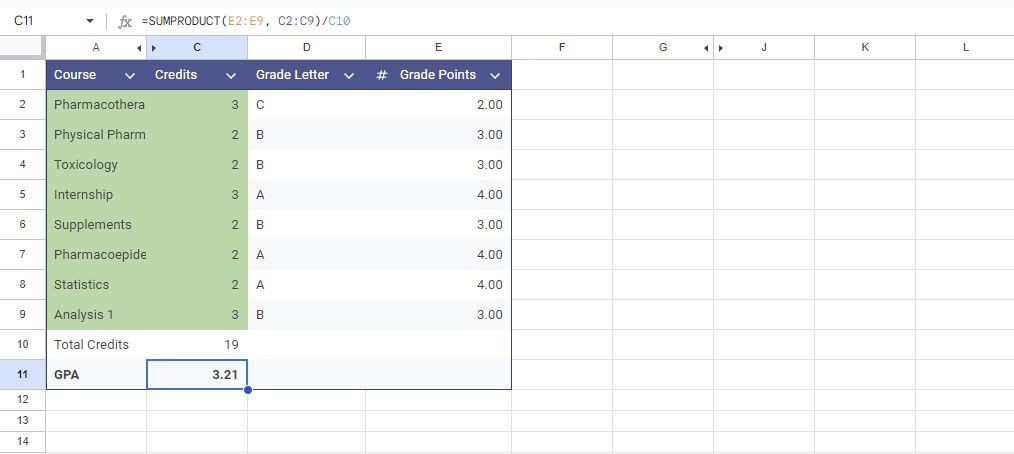
The spreadsheet looks cleaner now. Since I also don’t need the course ID in column B visible anymore, I’ll hide that too—no need to delete it, just in case I need it later in the semester. Now, with just a glance, the spreadsheet’s purpose—to calculate my GPA—is clear, without getting bogged down by unnecessary numbers and figures.
There are countless spreadsheet scenarios where certain cells are neither input nor output but serve as intermediary steps in your calculations. Hiding these cells can simplify the appearance of your spreadsheet, making it more user-friendly.
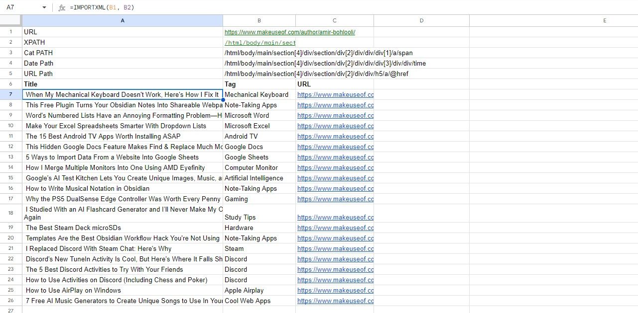
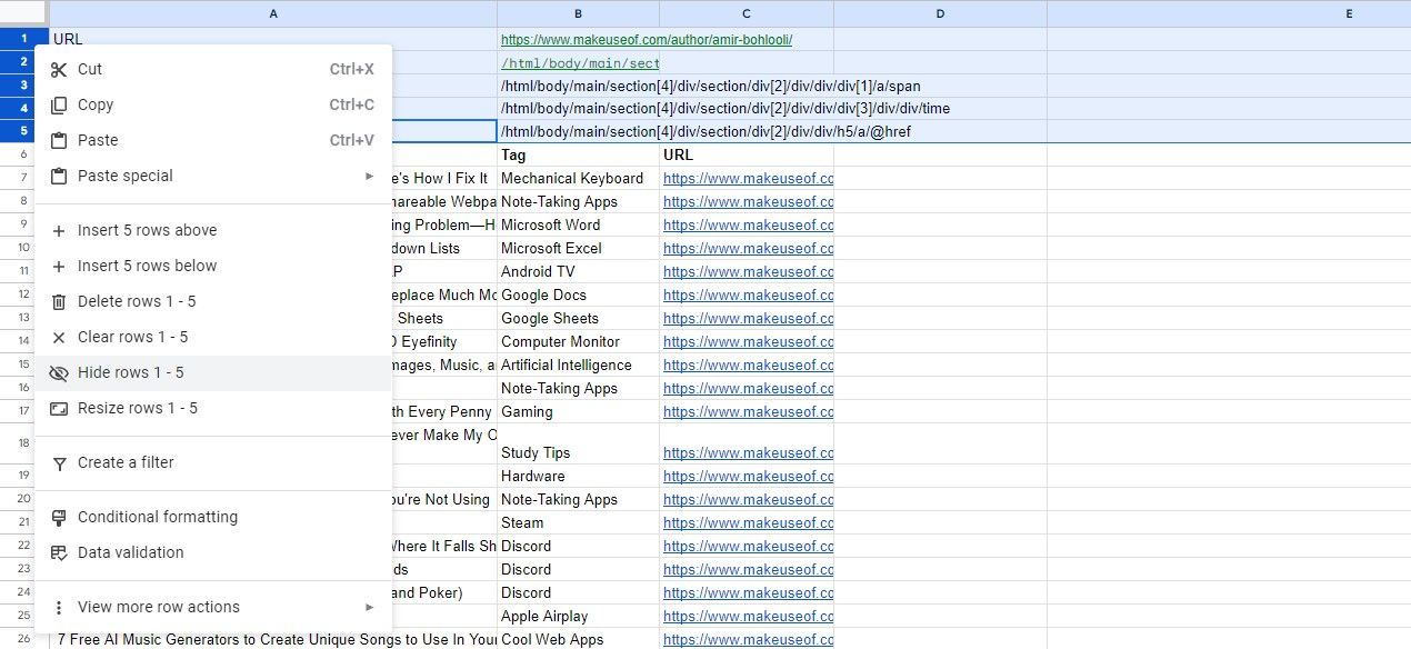
In another example, I used the IMPORTXML function to pull in my latest articles, along with their tags and URLs. The arguments for IMPORTXML are technical and clutter the top of the sheet. Since they’re in rows 1 to 5, hiding them makes the spreadsheet much more presentable.
Hiding rows follows the same steps: select the rows, right-click, and choose Hide row.
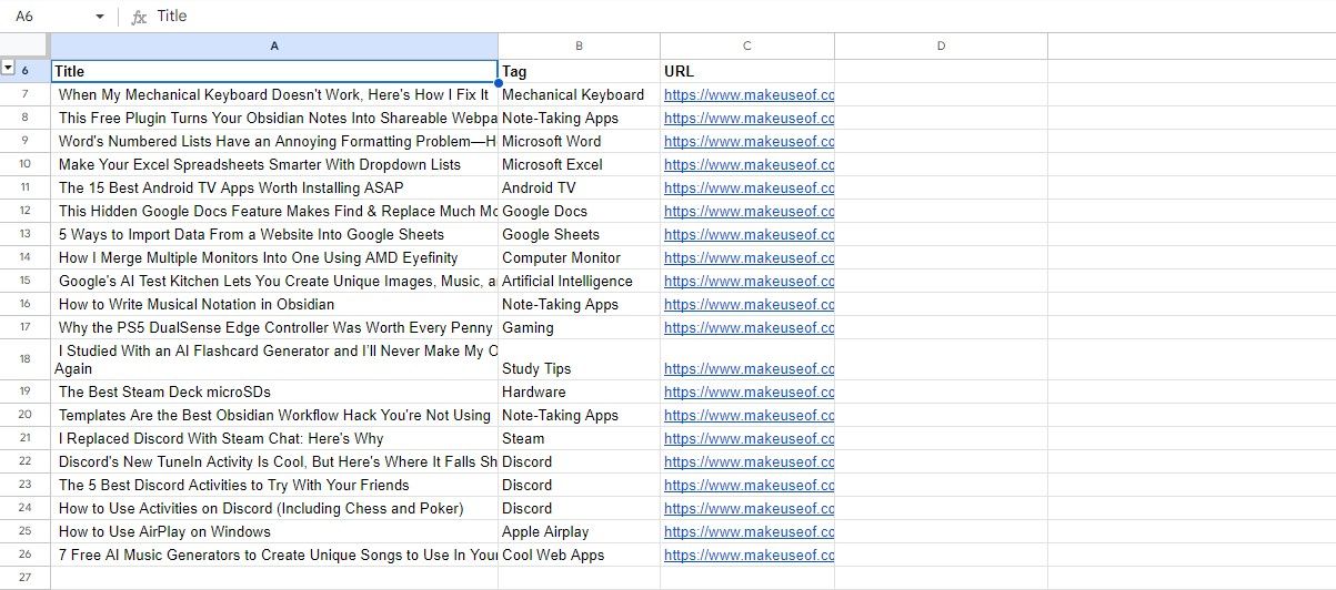
There you go! The table looks much simpler. Just like with hidden columns, you’ll see tiny arrows where the hidden rows are located.
How to Unhide Rows and Columns in Google Sheets
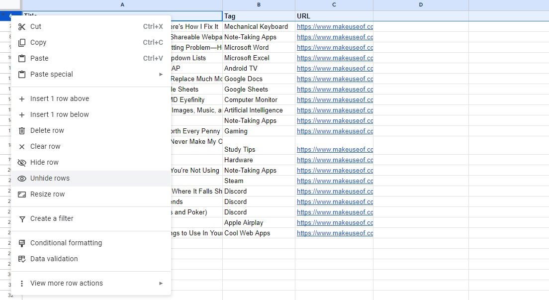
Hiding rows or columns is handy, but you might need to access those hidden cells again. Remember those tiny arrows that appear where a row or column was hidden? Just click on one, and the hidden rows or columns will reappear. Alternatively, you can right-click on an adjacent row or column and select Unhide columns or Unhide rows from the menu. That’s all there is to it.
Hiding and unhiding rows and columns in Google Sheets can greatly improve how you present your data. By decluttering your spreadsheet, you make it easier to focus on what really matters, whether you’re analyzing your academic performance or organizing work projects.

