Ever wondered why your Excel formulas sometimes produce unexpected results? It might be due to the order in which Excel performs calculations. This order is defined by the acronym PEMDAS. If you’re unfamiliar with PEMDAS or how it applies in Excel, here’s everything you need to know.
What is PEMDAS?
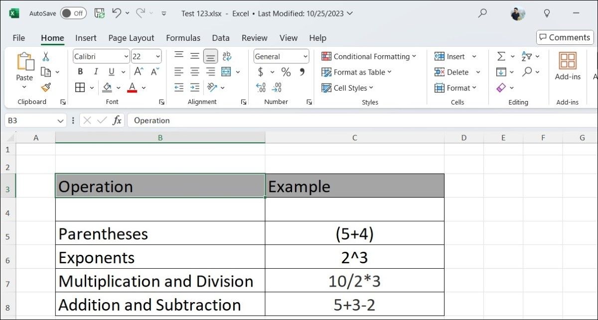
PEMDAS is an acronym that represents the order of operations in mathematics, which also applies to Excel formulas. Understanding this sequence is important, as it specifies how mathematical expressions are evaluated. The letters in PEMDAS stand for:
- Parentheses: Always first.
- Exponents: Powers and roots come next.
- Multiplication and Division: Equal priority and are processed from left to right.
- Addition and Subtraction: Also equal, done from left to right.
By understanding and applying PEMDAS in your Excel formulas, you can ensure that your calculations yield the intended results, thereby preventing errors and miscalculations.
The Order of Operations in Excel: A Closer Look
When working with formulas in Excel, the order of operations is crucial for ensuring accurate calculations. Here’s how the order of operations is applied in Excel formulas:
1. Parentheses
The first step in this order is evaluating expressions within parentheses. For instance, consider the formula =(5+3)*2. In this case, Excel first calculates the sum within the parentheses: 5+3 equals 8. Then, it multiplies that result by 2, yielding a final answer of 16.
2. Exponents
Following parentheses, Excel processes any exponents in the formula. An example would be =2^3 + 4. In this case, Excel calculates the exponent first, resulting in 2^3=8. After calculating the exponent, it adds 4 to the result, leading to a final value of 12.
3. Multiplication and Division
Next in line are multiplication and division, which Excel performs from left to right. For example, in the formula =10/2*3, Excel first divides 10 by 2, resulting in 5. It then multiplies 5 by 3, giving a final outcome of 15.
4. Addition and Subtraction
Lastly, addition and subtraction are handled from left to right. For example, in the formula =5+3-2, Excel first adds 5 and 3, which results in 8. It then subtracts 2 from 8, leading to a final answer of 6.
Complex Calculations
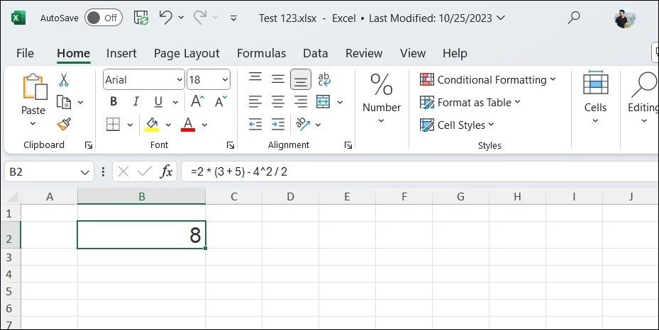
Now, let’s combine these concepts to see how Excel handles a complex calculation. For instance, take the formula =2*(3+5)-4^2/2. Here’s how Excel will calculate it:
- Parentheses are calculated first, so 3+5 becomes 8.
- Exponents are next, with 4^2 resulting in 16.
- Multiplication and division follow, leaving us with 2∗8−16/2, which simplifies to 16−8.
- Finally, addition and subtraction give us the answer: 8.
Still confused? You can use Excel’s Evaluate Formula feature to break down and understand formulas step by step.
Use Parentheses to Control the Order of Operations
While Excel does not allow you to change this standard order, you can manipulate this sequence by using parentheses. By enclosing parts of a formula in parentheses, you can easily prioritize specific operations in Excel.
For example, in the formula =5+2*3, Excel first multiplies 2 by 3, yielding 6, and then adds 5, resulting in 11. However, if you want to add first, you can use parentheses: =(5+2)*3. This computes to 7, which is then multiplied by 3 for a total of 21.
Using parentheses effectively can clarify your formulas, making them easier to read and ensuring that calculations are performed in the intended order. This is especially useful when writing complex formulas, as misplacing parentheses can lead to unexpected results.
Whether you’re working on simple calculations or intricate financial models, knowing the order of operations in Excel is vital. So, the next time you build a formula, take a moment to review the order of operations to avoid errors.


