The Top 6 Excel Formulas Every Office Worker Should Know

In a fast-paced office environment, time is everything. Inefficiencies in handling Excel can cost you precious hours, but what if you had the right tools at your fingertips to breeze through these challenges? These six essential Excel formulas are the shortcuts you need to save time, boost productivity, and make your daily workload feel a lot lighter.

1 IF and IFS

IF is one of the most widely used logical functions in Excel. It tests a condition and evaluates to either TRUE or FALSE. An IF formula has two possible outputs, one when the condition is TRUE and another when the condition is FALSE. It uses the syntax:

=IF(test, value_if_true, value_if_false) 

For more complex scenarios, Excel also offers the IFS function, which allows multiple conditions to be tested in a single formula without nesting/complicated syntax. IFS statements are written using the syntax:

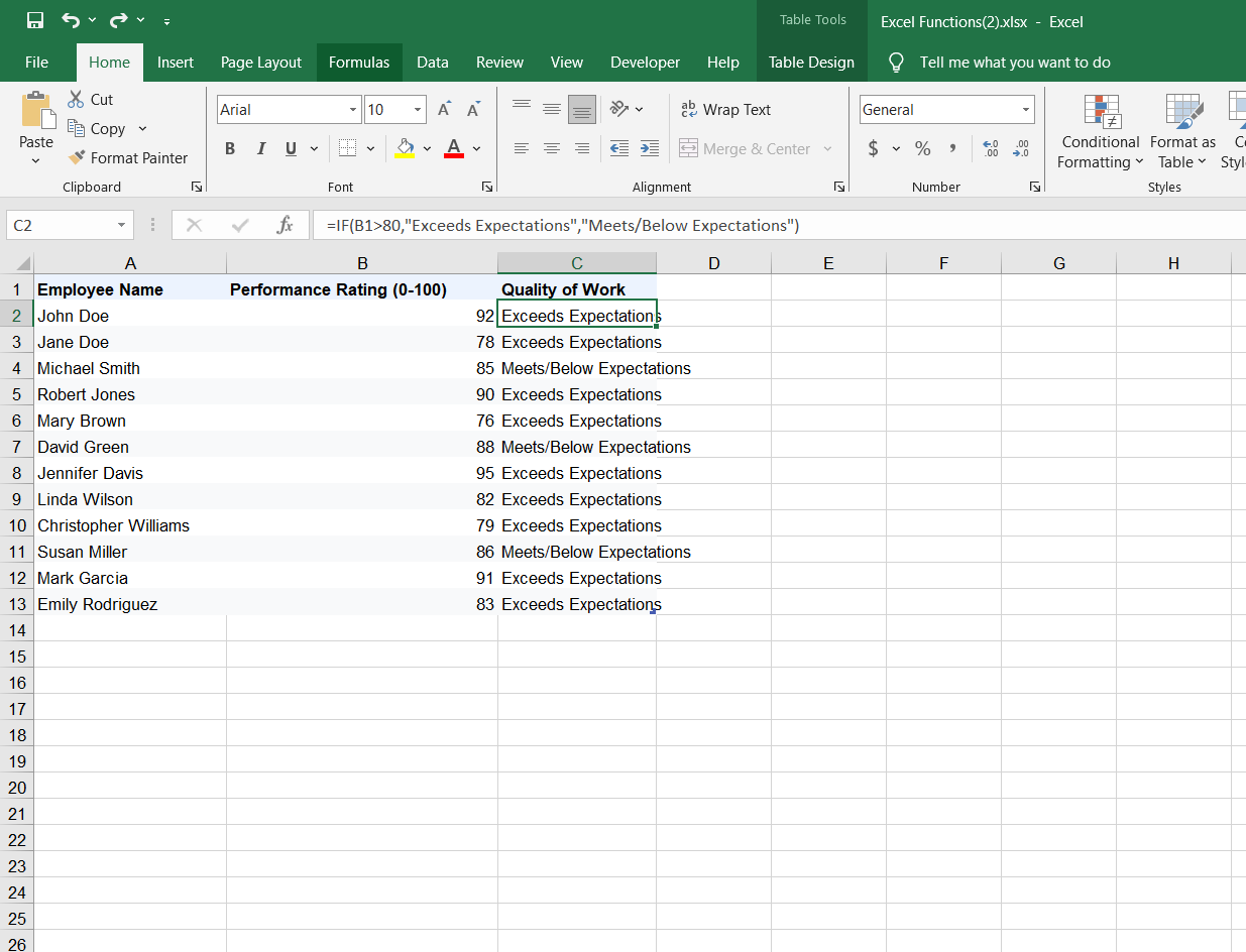
=IFS(condition1, value1, condition2, value2,...) 

These two functions can save a lot of time in an office environment. An HR specialist could use the IF function to automate employee performance reviews. A simple IF formula such as below can be used to classify employees based on their performance ratings:

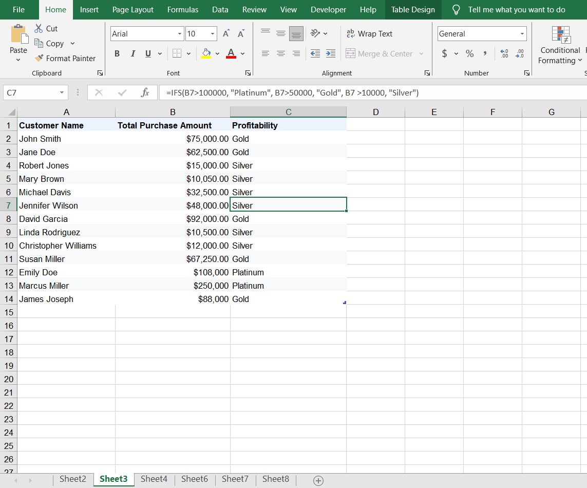
=IF(B1>80, "Exceeds Expectations", "Meets/Below Expectations") 

Or, the sales team could use the IFS statement to categorize customers based on their profitability:

=IFS(B2>100000, "Platinum", B2>50000, "Gold", B2>10000, "Silver") 

2 SUM and SUMIFS

As the name implies, the SUM function is used to add numbers together. It uses the syntax:

=SUM(num1, num2, ...) 

It can take numbers, cell references, and cell ranges as parameters. You can use the SUM function to quickly calculate totals for columns or rows of data. In a budget spreadsheet, you can use =SUM(B2:B10) to sum expenses over a specific period.

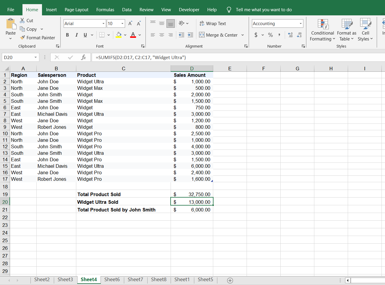
SUMIFS extends this functionality by allowing users to sum data based on multiple criteria. Its syntax is:

=SUMIFS(sum_range, criteria_range1, criteria1, [criteria_range2, criteria2], …) 

In practice, a SUMIFS formula can be used to add only the sales from a specific region, for a particular product, or by a particular salesperson. SUM and SUMIFS are just two of the SUM functions in Excel.

3 AGGREGATE

The AGGREGATE function combines different numerical aggregation functions into one. It performs calculations such as SUM, COUNT, MAX, and MIN while ignoring errors, hidden cells, and even other AGGREGATE and SUBTOTAL functions. The syntax is:

=AGGREGATE(function_num, options, ref, [k]) 

Where function_num represents the calculation to be performed, options determine what to ignore (e.g., hidden rows or errors), ref is the range of cells or array of cells to be aggregated, and k is an optional argument for certain functions.

AGGREGATE is especially useful in large datasets where standard functions like SUM or AVERAGE might be hindered by hidden data or errors.

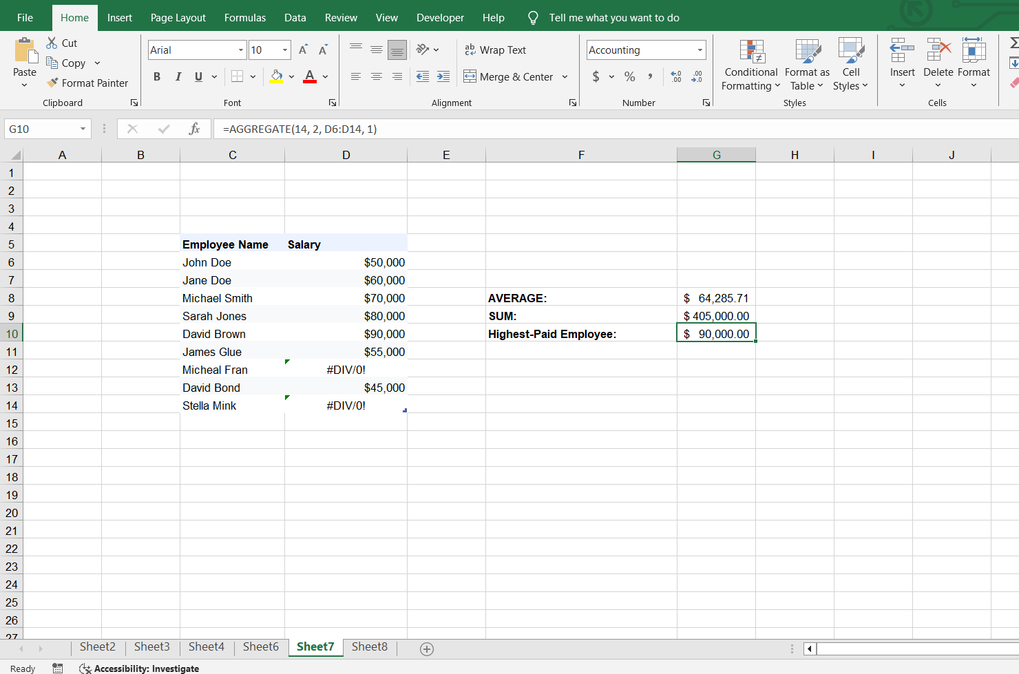
In the example below, AGGREGATE is applied to a table with errors to calculate the total, average, and highest salary received by employees. To calculate the highest salary, I used the formula:

=AGGREGATE(14, 2, D6:D14, 1) 

4 TRIM

The TRIM function performs data cleaning and removes extra spaces from text. This is especially useful for raw data that has been imported from an external source. It removes all extra spaces from text, including leading, trailing, and in-between spaces.

The syntax is simple:

=TRIM(text) 

It can come in handy for preparing a mailing list, cleaning up product descriptions, and organizing sales information.

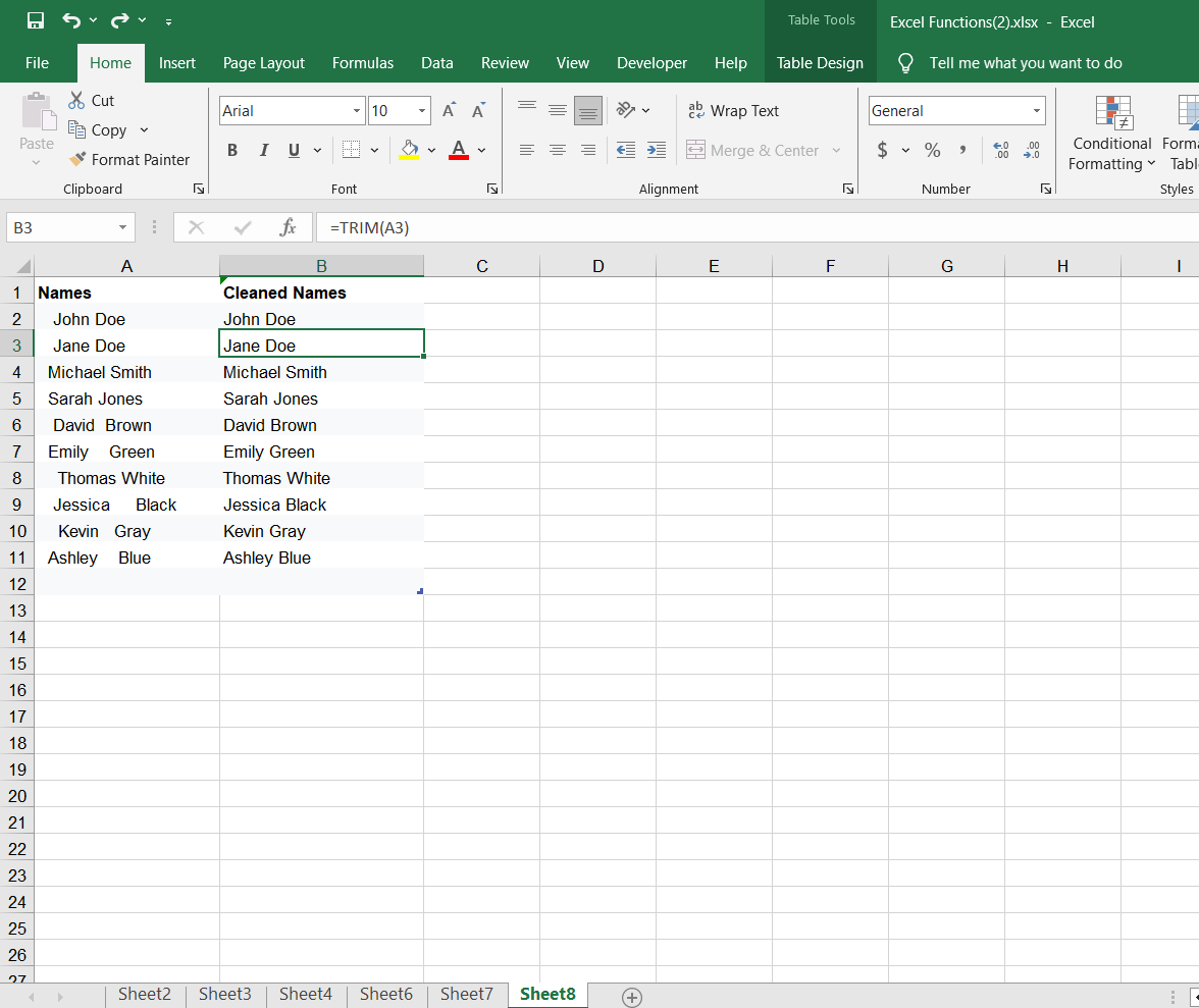
For instance, you can use TRIM to clean up leading, trailing, in-between spaces in a list of names, like in the screenshot below:

5 MIN and MAX

The MIN and MAX functions are easy to use and pretty straightforward. They take a series of numbers and find the smallest or largest value in the set. They can be used as an alternative to Excel’s AutoSum when the cells to be analyzed are scattered around the spreadsheet.

The syntax for MIN is:

=MIN(num1, num2, ...) 

and for MAX:

=MAX(num1, num2, ...) 

You can input numbers, cell references, or ranges for both functions.

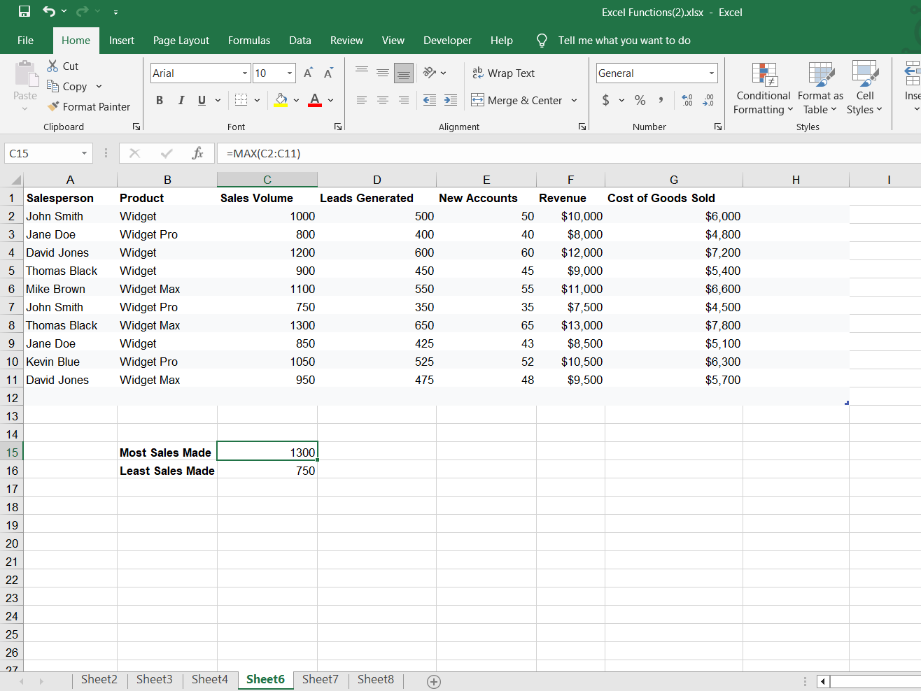
These functions are particularly useful for data analysis, such as identifying the highest and lowest sales figures in a report or monitoring the best and worst-performing products in a lineup. They are two of the essential Excel functions for beginners.

6 VLOOKUP and HLOOKUP

The VLOOKUP and HLOOKUP functions are used to look up values in Excel tables based on a predefined index value.

VLOOKUP (vertical lookup) searches for the lookup value in the first column of a defined range and returns the corresponding value in another column. HLOOKUP (horizontal lookup) searches for the lookup value in the top row of a table and returns a value from a different row in the same column.

Both formulas share a similar syntax:

=VLOOKUP(lookup_value, table_array, col_index_num, [range_lookup]
=HLOOKUP(lookup_value, table_array, row_index_num, [range_lookup]
 

Where the lookup_value is the number or text you want to search for, table_array is the range of cells that contain the lookup_value and the value to be returned, index_num is the column or row number that contains the return value, and the range_lookup is an optional parameter that specifies whether the function returns an approximate or exact match.

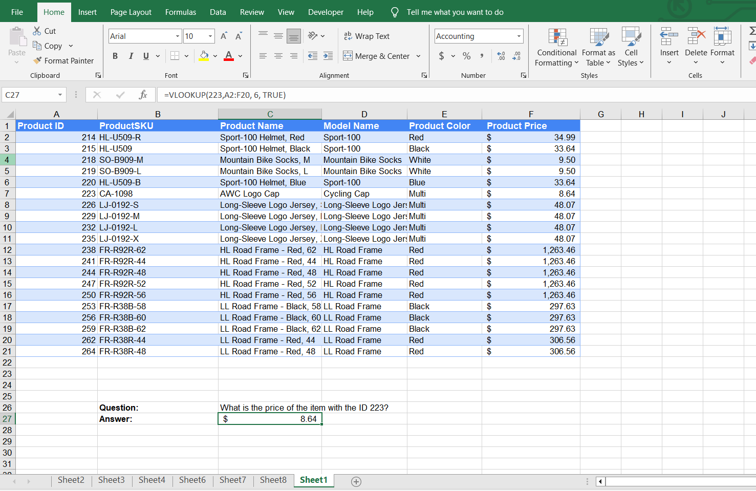
They are useful when working with large datasets with thousands of data items. For example, I can look through the inventory system to find the price of the product with the product ID 223 using the formula:

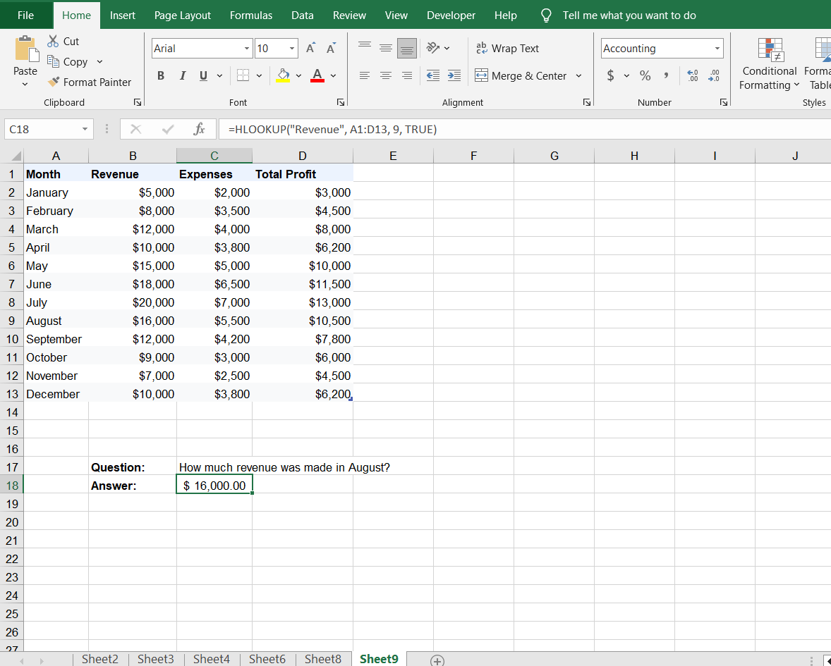
=VLOOKUP(223,A2:F20, 6, TRUE) 

HLOOKUP can be used to find data in tables structured by rows, such as sales for a specific month in a financial report. Using the following formula, I was able to determine how much revenue was made in the month of August.

=HLOOKUP("Revenue", A1:D13, 9, TRUE) 

From simple calculations like MIN and SUM to more advanced functions like VLOOKUP and HLOOKUP, these Excel formulas are essential for any office worker looking to boost their efficiency and stand out.