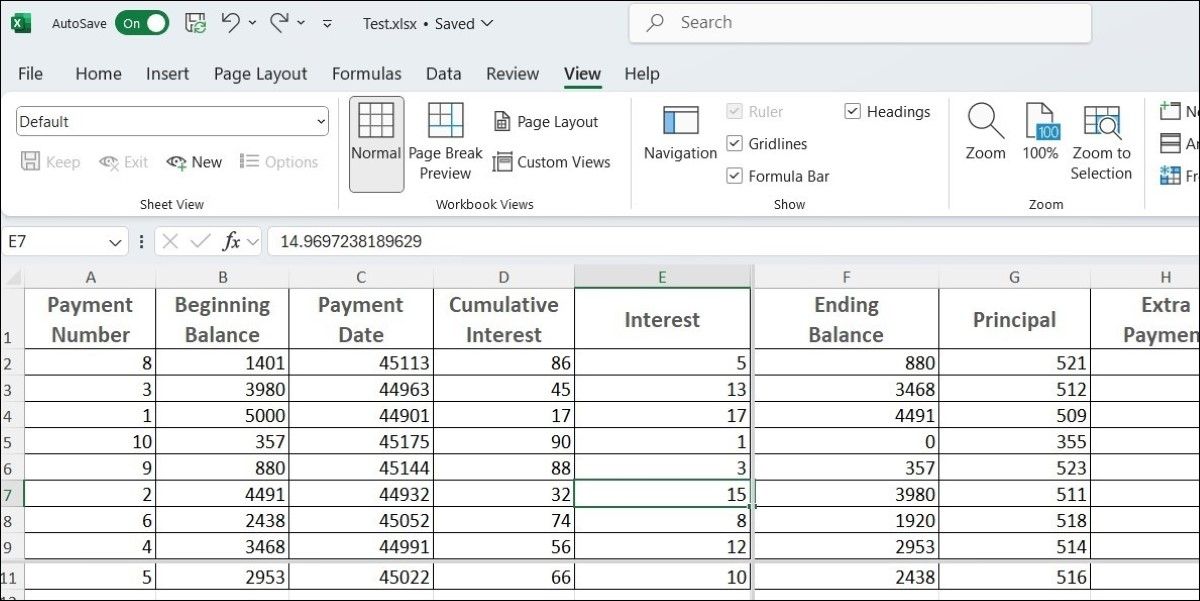
When working with large datasets, navigating between different sheets or windows can be time-consuming and inefficient. Fortunately, Excel’s split screen view offers a convenient solution for comparing data side by side. Here’s how to use it.
Viewing Worksheets in Split View
Excel’s split screen feature allows you to divide the window into two or four panes, making it easier to view different sections of the same worksheet or even multiple worksheets simultaneously.
Splitting the Window in a Single Worksheet
In Excel, you can split a worksheet into four parts by using the Split option. To do this, go to the View tab in your Excel workbook and click the Split button. This will divide your current worksheet into four sections, seperating them with thick gray lines.
You can then scroll each pane independently—both vertically and horizontally—allowing you to view different parts of the worksheet at the same time. If you prefer to split only horizontally, you can drag the vertical gray bar all the way to the left. For a vertical split, drag the horizontal bar to the top.
Comparing Different Sheets From the Same Workbook
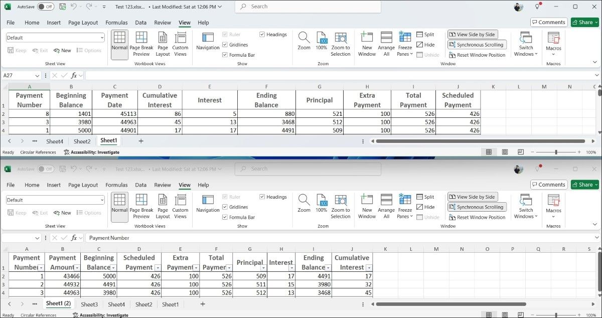
To view two different worksheets side by side, go to the View tab, and click New Window to open a second window of the same workbook. Then, go to the View tab again and click the View Side by Side button.
Excel will arrange the two windows, one above the other. By default, both windows will scroll simultaneously, which makes it easier to spot differences between the worksheets. If you prefer to scroll independently, simply click the Synchronous Scrolling button in the View tab to deactivate it.
Comparing Worksheets From Different Workbooks
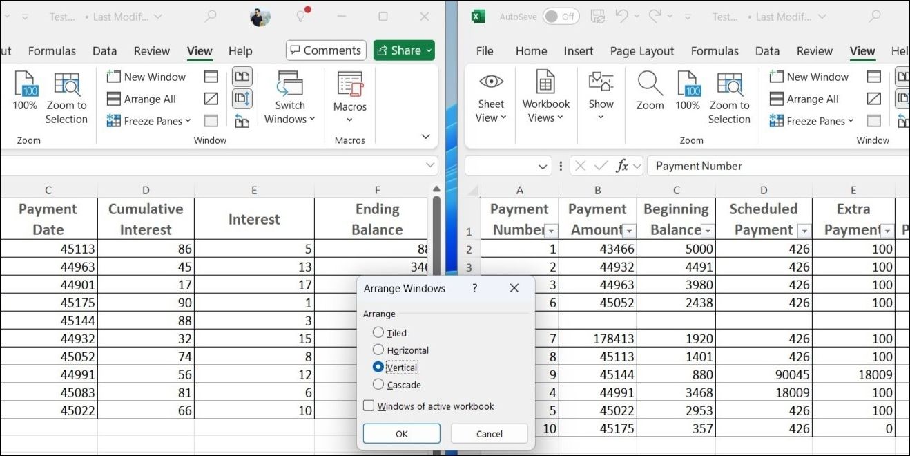
If you need to compare worksheets from two different workbooks, first open both workbooks. Then, navigate to the View tab and select Compare Side by Side. If multiple files are open, a dialog box will appear, prompting you to choose which workbook you want to compare with the active one.
Once in side-by-side view, you can scroll through each workbook independently or use Synchronous Scrolling for simultaneous navigation. Additionally, if you want to adjust the layout, click the Arrange All button to switch between horizontal and vertical arrangements.
Once you are done comparing your data side by side in Excel’s split screen view, you may want to remove the split to return to your original view. To do so, all you have to do is go to the View tab again and click the Split button again.
Tips for Using Split Screen Effectively
If you need to use Excel’s split screen feature regularly, it’s a good idea to familiarize yourself with these tips to maximize your efficiency.
Use Keyboard Shortcuts
Keyboard shortcuts in Excel can save you time when using the split screen feature. For instance, you can press Alt + W + S to quickly enable or disable the Split feature in Excel.
Reset Excel’s Split View
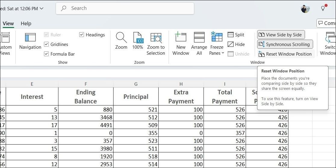
After resizing workbook windows or rearranging your split view, you may find that your layout is not as effective as it once was. To restore the default settings, simply click the Reset Window Position button in the View tab.
Save Your Split Screen Presets
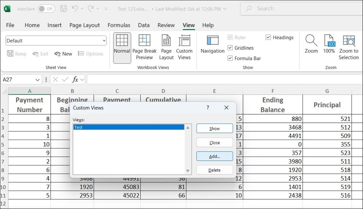
Excel’s Custom Views feature is a powerful tool for saving your preferred layouts, including any split screen settings. To create a preset, navigate to the View tab, select Custom Views, and then click Add to name and save your current layout.
Once saved, you can click the Custom Views option, select your desired view, and hit Show to apply it instantly.
The ability to view multiple sections of your spreadsheet simultaneously provides the clarity and organization needed for effective data comparison. This is especially useful for tasks that require attention to detail, such as analyzing financial reports, comparing sales figures, or reviewing project timelines. The best part is that using Excel’s split screen feature isn’t complicated once you get the hang of it.

